The chopper meets an R-L load
Slide 37 is the front half of the buck: $T_1$ (an IGBT) and the freewheeling diode $D_1$. Dr. Xu's margin note calls it a voltage chopper: its output $v_o$ is $V_d$ while $T_1$ is on and 0 while $D_1$ freewheels. There's no capacitor this time. The load is an inductor in series with a resistor, and he labelled it a first-order filter.
One-quadrant means $I_o > 0$ and $V_o > 0$ only, because $T_1$ and $D_1$ each conduct one way. The two-quadrant chopper on slide 62 adds negative current ($I_o = \pm$); that's next lecture.
- $T_1$ on, so $v_o = V_d$ (class note). KVL around the load: $V_d = L\frac{di_o}{dt} + Ri_o$. Starting at $I_{\min}$ and heading for $V_d/R$: $$i_o(t) = \frac{V_d}{R}\left(1 - e^{-t/\tau}\right) + I_{\min}e^{-t/\tau}, \quad 0 \le t < t_{on} \quad (1)$$
- $D_1$ on, so $v_o = 0$: $0 = L\frac{di_o}{dt} + Ri_o$. Starting at $I_{\max}$, heading for 0, clock restarted at $t_{on}$: $$i_o(t) = I_{\max}e^{-(t - t_{on})/\tau}, \quad t_{on} \le t < T_s \quad (2)$$
- Both come from one template, slide 38's note (Dr. Xu wrote "ELE202" beside it): $$\tau\frac{dx}{dt} = -x + b \;\Rightarrow\; x(t) = x_0e^{-t/\tau} + b\left(1 - e^{-t/\tau}\right), \qquad \tau = \frac{L}{R}$$ $x_0 = x(0)$ is where you start, $b = x(\infty)$ is where you're heading. Divide the on-time KVL by R and you get exactly this form with $b = V_d/R$. Class note: $I_{\min} > 0$. With an R-L load the current decays toward zero but never reaches it, so this load is always in continuous current mode.
In the buck, C held $V_o$ constant, so $v_L$ was constant and $i_L$ was a ramp. Here $v_L = v_o - Ri_o$ moves as $i_o$ moves, so the slope keeps changing. Slide 38: "$i_o$ does not increase or decrease linearly!" When $\tau \gg T_s$ each interval only uses the first, nearly straight bit of the exponential. The hero demo at the top shows both cases.
$T_1$ has just turned off and $D_1$ picks up the current. What does $i_o$ do?
With $D_1$ on, $v_o = 0$ and the load is L discharging into R: $0 = L\frac{di_o}{dt} + Ri_o$, so $i_o = I_{\max}e^{-(t - t_{on})/\tau}$. It heads for 0 (the final value b), not below: nothing in the loop pushes it negative. An inductor current can't jump, so "drops to zero at once" is out.
$I_{\max}$ and $I_{\min}$ in steady state
Dr. Xu wrote "in steady state" twice on slide 39: every period starts where the last one ended. That gives two conditions for two unknowns.
- End of the on-time, from (1): $$i_o(t_{on}) = I_{\max} = \frac{V_d}{R}\left(1 - e^{-t_{on}/\tau}\right) + I_{\min}e^{-t_{on}/\tau} \quad (3)$$
- End of the period, from (2): $$i_o(T_s) = I_{\min} = I_{\max}e^{-(T_s - t_{on})/\tau} \quad (4)$$
- The step the slide skips: put (4) into (3). The two exponentials multiply to $e^{-T_s/\tau}$: $$I_{\max} = \frac{V_d}{R}\left(1 - e^{-t_{on}/\tau}\right) + I_{\max}e^{-T_s/\tau} \;\Rightarrow\; I_{\max}\left(1 - e^{-T_s/\tau}\right) = \frac{V_d}{R}\left(1 - e^{-t_{on}/\tau}\right)$$
- $$\boxed{I_{\max} = \frac{V_d}{R}\,\frac{1 - e^{-t_{on}/\tau}}{1 - e^{-T_s/\tau}}}$$
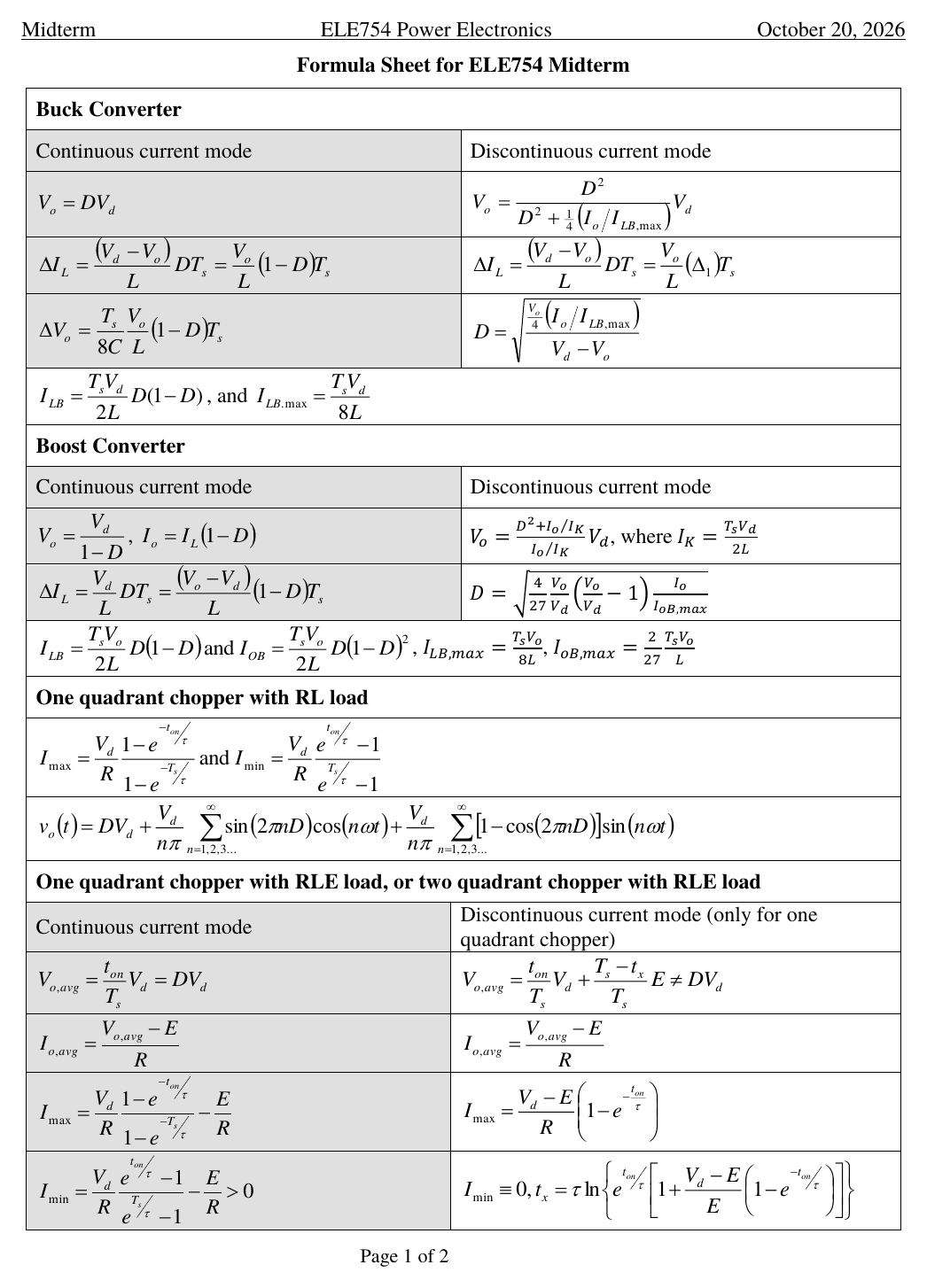
- Back into (4), then multiply top and bottom by $e^{T_s/\tau}$: $$I_{\min} = \frac{V_d}{R}\,\frac{\left(1 - e^{-t_{on}/\tau}\right)e^{-(T_s - t_{on})/\tau}}{1 - e^{-T_s/\tau}} \;\Rightarrow\; \boxed{I_{\min} = \frac{V_d}{R}\,\frac{e^{t_{on}/\tau} - 1}{e^{T_s/\tau} - 1}}$$ Both boxes are on your formula sheet, row "One quadrant chopper with RL load". Watch the signs: $I_{\max}$ has negative exponents, $I_{\min}$ positive ones.
Example II: an R-L load at 75%
A one-quadrant chopper with an R-L load: $V_d = 120$ V, $f_{sw} = 1$ kHz, $L = 4.5$ mH, $R = 1.5\ \Omega$, $D = 0.75$. Find (1) the current ripple $\Delta I$ and (2) the averages $I_o$ and $V_o$.
Try it on paper first, then reveal one step at a time.
- $\tau = \frac{L}{R} = \frac{4.5\text{ mH}}{1.5\ \Omega} = 3$ ms, $\;T_s = \frac{1}{f_{sw}} = 1$ ms, $\;t_{on} = DT_s = 0.75$ ms.
- $$I_{\max} = \frac{120}{1.5}\cdot\frac{1 - e^{-0.75/3}}{1 - e^{-1/3}} = 80\times\frac{0.2212}{0.2835} = 62.4\text{ A}$$
- $$I_{\min} = 80\times\frac{e^{0.25} - 1}{e^{1/3} - 1} = 80\times\frac{0.2840}{0.3956} = 57.4\text{ A}$$
- ΔI = I_max − I_min = 4.99 A (the slide prints 4.9 A; see the note below).
- $V_{o,avg} = DV_d = 0.75\times120 = $ 90 V, and $I_{o,avg} = \frac{V_{o,avg}}{R} = \frac{90}{1.5} = $ 60 A, because the inductor has no dc voltage drop.
Unrounded, $I_{\max} = 62.43$ A and $I_{\min} = 57.44$ A. The slide rounds $I_{\min}$ up to 57.5 A, so its $\Delta I = 62.4 - 57.5 = 4.9$ A; the true ripple is 4.99 A. A ripple is a small difference of two big numbers, so on the exam keep four figures until you subtract.
Two class notes on this example
Next to step 5 Dr. Xu wrote $\frac{V_d - V_o}{L}t_{on}$ and put an X through it. That formula needs a constant voltage on the far side of L: the buck's capacitor, or a battery ("$V_{bat}$ = const"). Here the far side is $Ri_o$, which moves. Because $\tau = 3$ ms is three times $T_s$, the curves are nearly straight and the buck-style estimate $\frac{120 - 90}{4.5\text{ mH}}\times0.75$ ms $= 5.0$ A lands close, but it's an approximation. Use $I_{\max} - I_{\min}$.
He drew the dc equivalent circuit: averaged over a period, $V_L = 0$, so L is a short for dc and $I_{o,avg} = V_{o,avg}/R$ exactly. The slide's second route, $I_{o,avg} \approx \frac{I_{\max} + I_{\min}}{2}$, he circled and marked "not equal": exponential segments aren't symmetric, so the midpoint is only close when R is very small ($\tau \gg T_s$). Here it's 59.93 A.
A one-quadrant chopper drives an R-L load: $V_d = 200$ V, $D = 0.6$, $R = 2\ \Omega$, $L = 5$ mH, $f_{sw} = 2$ kHz. You find $I_{\max} = 62.38$ A and $I_{\min} = 57.59$ A. What is the average load current?
$V_{o,avg} = DV_d = 120$ V and the inductor drops no average voltage, so $I_{o,avg} = 120/2 = 60$ A whatever L is. The midpoint, 59.98 A, is close because $\tau = 2.5$ ms is five times $T_s = 0.5$ ms, but it isn't exact. $V_d/R$ is where the current would end up if $T_1$ stayed on forever.
Add a back emf: the dc motor load
Slide 43 swaps the load for a dc motor's equivalent circuit: armature inductance L, armature resistance R and back emf E. Dr. Xu sketched where you'd meet it: a 12 V PC fan, chopped by a MOSFET with a freewheeling diode across the motor. He labelled E a constant voltage source. The motor's speed changes slowly compared with $T_s$, so over one period E doesn't move.
Every KVL loop now has an extra E (the red boxes Dr. Xu drew on slide 44): $v_o = L\frac{di_o}{dt} + Ri_o + E$.
- $T_1$ on: $V_d = L\frac{di_o}{dt} + Ri_o + E$, so the current heads for $\frac{V_d - E}{R}$: $$i_o(t) = \frac{V_d - E}{R}\left(1 - e^{-t/\tau}\right) + I_{\min}e^{-t/\tau} \quad (1)$$
- $D_1$ on: $0 = L\frac{di_o}{dt} + Ri_o + E$, so it heads for $-\frac{E}{R}$, which is below zero: $$i_o(t) = -\frac{E}{R}\left(1 - e^{-(t - t_{on})/\tau}\right) + I_{\max}e^{-(t - t_{on})/\tau} \quad (2)$$
- Same steady-state move as slide 39, and E comes out as one shift: $$I_{\max} = \frac{V_d}{R}\,\frac{1 - e^{-t_{on}/\tau}}{1 - e^{-T_s/\tau}} - \frac{E}{R}, \qquad I_{\min} = \frac{V_d}{R}\,\frac{e^{t_{on}/\tau} - 1}{e^{T_s/\tau} - 1} - \frac{E}{R}$$ Why a plain shift: the circuit is linear, so the response to the pulse train and the response to E add. A constant E on its own drives a constant $-E/R$ through the load.
- Averages (slide 44): $V_{o,avg} = \frac{\text{Area }A_1}{T_s} = DV_d$ still, and the dc circuit gives $$I_{o,avg} = \frac{V_{o,avg} - E}{R}$$ These four are the CCM column of the "RLE load" row on your formula sheet. Its $I_{\min}$ line ends in "$> 0$": that's the condition for using the column at all.
Example II's numbers with $E = 30$ V (magenta) against $E = 0$ (blue): the whole waveform drops by $E/R = 20$ A. The ripple stays 4.99 A and the average falls from 60 A to 40 A.
Example II (120 V, 75%, 4.5 mH, 1.5 Ω) now drives a motor with $E = 30$ V. What happens to $I_{\max}$, $I_{\min}$ and $\Delta I$?
Subtract $E/R = 30/1.5 = 20$ A from both: 42.43 A and 37.44 A. The shape depends on $V_d$, D, $\tau$ and $T_s$, none of which changed, so $\Delta I = 4.99$ A. The average drops to $(90 - 30)/1.5 = 40$ A. Keep raising E and $I_{\min}$ hits zero. That's the next section.
When the current runs out: DCM
Raise E (a lightly loaded motor spins faster) and $I_{\min} = (\text{R-L value}) - E/R$ keeps falling. The CCM formula happily returns a negative number, but the current can't follow: $T_1$ and $D_1$ only conduct one way. So the current reaches zero at some instant $t_x$ and stays there until $T_1$ turns on again. That's discontinuous current mode, with three intervals (slide 46):
- $0 \le t < t_{on}$: $T_1$ on, $v_o = V_d$, current rises from zero.
- $t_{on} \le t < t_x$: $D_1$ on, $v_o = 0$, L releases its energy to the load.
- $t_x \le t < T_s$: both off and $i_o = 0$. No current means no drop on R or L (class: "$I_oR = 0$", "$V_L = 0$"), so $v_o = E$.
Example III. Dashed: the curve the CCM formulas assume, which would dip to −84 A. The real current stops at zero at $t_x$, and from there the output sits at E.
Average output (slide 46): $$V_{o,avg} = \frac{\text{Area }A_1 + \text{Area }A_2}{T_s} = \frac{t_{on}}{T_s}V_d + \frac{T_s - t_x}{T_s}E \;\ne\; DV_d$$ Dr. Xu marked $A_1$ "due to $V_d$", $A_2$ "due to E", and $t_x$ "unknown". So DCM needs one more formula.
- Each period now starts at zero, so put $I_{\min} = 0$ in (1): $$I_{\max} = \frac{V_d - E}{R}\left(1 - e^{-t_{on}/\tau}\right) \quad (3)$$ Not the CCM $I_{\max}$. Once you know it's DCM, recompute it.
- At $t_x$ the current in (2) reaches zero: $$0 = -\frac{E}{R}\left(1 - e^{-(t_x - t_{on})/\tau}\right) + I_{\max}e^{-(t_x - t_{on})/\tau} \quad (4)$$
- The skipped algebra: collect the exponential terms. $$\left(I_{\max} + \frac{E}{R}\right)e^{-(t_x - t_{on})/\tau} = \frac{E}{R} \;\Rightarrow\; t_x - t_{on} = \tau\ln\left(1 + \frac{RI_{\max}}{E}\right)$$
- Use (3) for $RI_{\max}$ and fold $t_{on}$ into the log as $\tau\ln e^{t_{on}/\tau}$: $$\boxed{t_x = \tau\ln\left\{e^{t_{on}/\tau}\left[1 + \frac{V_d - E}{E}\left(1 - e^{-t_{on}/\tau}\right)\right]\right\}}$$ $t_x$ is measured from the start of the period, not from turn-off. The DCM column of your formula sheet has (3), $I_{\min} \equiv 0$, this $t_x$ and $V_{o,avg}$.
- Assume CCM and compute $I_{\min}$ with the CCM formula. $I_{\min} > 0$: CCM. $I_{\min} < 0$: DCM.
- Or assume DCM and compute $t_x$. $t_x > T_s$: CCM, the current never ran out. $t_x < T_s$: DCM.
- If it's DCM, throw away the CCM $I_{\max}$ and $V_{o,avg} = DV_d$. Use $I_{\min} \equiv 0$, $I_{\max} = \frac{V_d - E}{R}\left(1 - e^{-t_{on}/\tau}\right)$, $t_x$, then $V_{o,avg}$ and $I_{o,avg} = \frac{V_{o,avg} - E}{R}$.
The two checks always agree; the bench computes both. With $E = 0$ the log blows up ($t_x \to \infty$): an R-L load is always CCM.
Example III (slides 49 to 51)
A one-quadrant chopper drives a dc motor: $V_d = 110$ V, $f_{sw} = 400$ Hz, $L = 0.2$ mH, $R = 0.25\ \Omega$, $D = 0.5$, $E = 40$ V. Find (1) the mode, (2) $I_{\max}$ and $I_{\min}$, (3) the averages $I_o$ and $V_o$.
- $\tau = 0.8$ ms, $T_s = 2.5$ ms, $t_{on} = 1.25$ ms. Assume CCM: $$I_{\min} = 440\times\frac{e^{1.5625} - 1}{e^{3.125} - 1} - 160 = 76.25 - 160 = -84\text{ A} < 0$$ so DCM.
- $I_{\max} = \frac{110 - 40}{0.25}\left(1 - e^{-1.5625}\right) = 280\times0.7904 = $ 221.3 A and $I_{\min} = 0$ (the slide prints 221.2 A).
- $t_x = 0.8\text{ ms}\times\ln\left\{e^{1.5625}\left[1 + \frac{70}{40}(0.7904)\right]\right\} = 0.8\text{ ms}\times\ln 11.37 = $ 1.945 ms, less than $T_s = 2.5$ ms: DCM confirmed the second way.
- $V_{o,avg} = \frac{1.25}{2.5}\times110 + \frac{2.5 - 1.945}{2.5}\times40 = 55 + 8.88 = $ 63.9 V (slide: 64 V).
- $I_{o,avg} = \frac{63.9 - 40}{0.25} = $ 95.5 A. The slide's rounded 64 V gives 96 A: dividing a small difference by a small R magnifies rounding, so carry the digits.
You assume CCM for a chopper driving a motor, and the CCM formula gives $I_{\min} = -84$ A. What does that tell you?
Neither $T_1$ nor $D_1$ can carry negative current, so $i_o \ge 0$ always. A negative $I_{\min}$ means the real current reached zero before the period ended. Recompute $I_{\max}$ with $I_{\min} \equiv 0$ and find $t_x$. Sending power back to $V_d$ needs the two-quadrant chopper.
In DCM, between $t_x$ and $T_s$, what is $v_o$?
At $t_x$ the current is zero and $D_1$ turns off; $T_1$ is still off. KVL with $i_o = 0$: $v_o = L\frac{di_o}{dt} + Ri_o + E = E$. That's area $A_2$, the reason $V_{o,avg} > DV_d$ in DCM: 63.9 V instead of 55 V in Example III.
Run the chopper yourself
Everything here comes from the slide formulas, so it doubles as an answer checker. Load a preset, then push it around: raise E until the badge flips to DCM, shrink L and watch the ripple grow, or watch which harmonics the load lets through.
Show the numbers
| h | |Voh| (V) | Zh (Ω) | |Ioh| (A) | rms (A) |
|---|
Fourier series in one page
Any periodic waveform is a dc value plus sinusoids at whole multiples of its frequency. Slide 52's definitions, with $\omega = 2\pi/T$: $$f(t) = f_0 + \sum_{n=1}^{\infty}a_n\cos(n\omega t) + \sum_{n=1}^{\infty}b_n\sin(n\omega t)$$ $$f_0 = \frac{1}{T}\int_0^T f(t)\,dt, \qquad a_n = \frac{2}{T}\int_0^T f(t)\cos(n\omega t)\,dt, \qquad b_n = \frac{2}{T}\int_0^T f(t)\sin(n\omega t)\,dt$$ Each pair combines into one sinusoid, $c_n\sin(n\omega t + \theta_n)$, with $c_n = \sqrt{a_n^2 + b_n^2}$ (Dr. Xu: "magnitude") and $\theta_n = \tan^{-1}(a_n/b_n)$ ("phase angle"). n = 1 is the fundamental; the rest are harmonics.
Slide 53's square wave swings $\pm V_m$: $$v_o = \frac{4V_m}{\pi}\left(\sin\omega t + \frac{1}{3}\sin 3\omega t + \frac{1}{5}\sin 5\omega t + \dots\right)$$ Only odd harmonics. Class note: the wave is half-wave symmetric, $f(t + T/2) = -f(t)$, and that cancels every even harmonic. The amplitudes fall as $1/n$, so three terms already look square (slide 54).
Extra if you have time: push the builder to 25 terms. The overshoot at each edge never shrinks below about 9% of the jump (the Gibbs effect); it just gets narrower.
The chopper's harmonics
Slide 55 applies this to the chopper output: $v_o = V_d$ for $0 \le t < DT_s$ and 0 for the rest of the period, with D anywhere from 0 to 1 (class note). Step through slide 56, with the algebra it skips.
- dc: $$V_{o,dc} = \frac{1}{T_s}\int_0^{DT_s}V_d\,dt = DV_d$$
- $a_n$: only the pulse contributes. $$a_n = \frac{2}{T_s}\int_0^{DT_s}V_d\cos(n\omega t)\,dt = \frac{2V_d}{n\omega T_s}\Big[\sin(n\omega t)\Big]_0^{DT_s} = \frac{2V_d}{n\omega T_s}\sin(n\omega DT_s)$$ The slide's middle step writes $\frac{1}{n\omega}\int\dots d(\omega t)$; with $\frac{1}{n\omega}$ in front the variable should be $d(n\omega t)$. Its next line is right.
- The key substitution: $\omega = 2\pi f_{sw} = 2\pi/T_s$, so $\omega T_s = 2\pi$. Then $n\omega DT_s = 2\pi nD$ and $\frac{2V_d}{n\omega T_s} = \frac{V_d}{n\pi}$: $$\boxed{a_n = \frac{V_d}{n\pi}\sin(2\pi nD)}$$
- $b_n$ the same way: $$b_n = \frac{2V_d}{n\omega T_s}\Big[-\cos(n\omega t)\Big]_0^{DT_s} \;\Rightarrow\; \boxed{b_n = \frac{V_d}{n\pi}\left[1 - \cos(2\pi nD)\right]}$$ Class note: both are functions of D (times $V_d$), not of $T_s$. Together they're the $v_o(t)$ row on your formula sheet: $a_n$ is the cosine coefficient, $b_n$ the sine one.
- Not on the sheet, and it saves time: $$V_{on} = \sqrt{a_n^2 + b_n^2} = \frac{2V_d}{n\pi}\left|\sin(n\pi D)\right|$$ With $x = n\pi D$: $\sin^2 2x + (1 - \cos 2x)^2 = 2 - 2\cos 2x = 4\sin^2 x$. So $V_{on} = 0$ whenever nD is a whole number. In Example IV ($D = 0.4$) the 5th and 10th vanish.
A chopper runs at $D = 0.25$. Which harmonic of $v_o$ is zero?
$V_{on} = \frac{2V_d}{n\pi}|\sin(n\pi D)|$ is zero when nD is a whole number: n = 4, 8, 12 and so on. All the even harmonics vanish together only at $D = 0.5$. Load "Harmonics problem" on the bench (D = 0.25) to see the gaps at 4 and 8.
Each harmonic sees its own impedance (slide 57)
The load is linear, so treat each harmonic as its own sinusoidal source and add the responses (superposition). Slide 57 draws three equivalent circuits:
Dr. Xu's note on the dc circuit: no voltage drop on the inductor.
- dc: L is a short, so $I_{o,dc} = V_{o,dc}/R$.
- h-th harmonic: L has reactance $h\omega_1L$, with $\omega_1 = 2\pi f_{sw}$: $$Z_h = \sqrt{R^2 + (h\omega_1L)^2}, \qquad I_{oh} = \frac{V_{oh}}{Z_h}$$
- Phase, if a question asks: the current lags its voltage by $\tan^{-1}(h\omega_1L/R)$. Slide 58's margin phasor note: $V\angle\theta_v = I\angle\theta_i\cdot Z$.
The sheet gives the $v_o(t)$ series only (and writes $\frac{V_d}{n\pi}$ outside the sum, as slide 56 does; the n belongs inside). You bring: $V_{on} = \sqrt{a_n^2 + b_n^2}$, $\omega = 2\pi f_{sw}$, $Z_h$, $I_{oh} = V_{oh}/Z_h$, and rms = peak/√2. $Z_h$ grows with h, so the R-L load passes low harmonics and crushes high ones. That's the "first-order filter" from slide 37, written again on slide 61.
Example IV: $R = 10\ \Omega$, $L = 1$ mH, $f_{sw} = 1$ kHz. What impedance does the 3rd harmonic see?
$\omega_3 = 3\omega_1$, so $X_3 = 3\times2\pi\times1000\times0.001 = 18.85\ \Omega$ and $Z_3 = \sqrt{100 + 355.3} = 21.34\ \Omega$. R and X add as phasors, not arithmetically. 11.81 Ω is $Z_1$. Only the dc circuit drops L.
Example IV: harmonics of an R-L load
A one-quadrant chopper with an R-L load: $V_d = 100$ V, $D = 0.4$, $R = 10\ \Omega$, $L = 1$ mH, $f_{sw} = 1$ kHz. Find the harmonic components of (1) $v_o$ and (2) $i_o$, up to the 5th. Try it, then reveal.
- dc: $V_{o,dc} = DV_d = 40$ V and $I_{o,dc} = 40/10 = 4$ A.
- n = 1, with $\frac{V_d}{\pi} = 31.83$: $a_1 = 31.83\sin(0.8\pi) = 31.83\times0.5878 = 18.71$ and $b_1 = 31.83\left[1 - \cos(0.8\pi)\right] = 31.83\times1.809 = 57.58$, so $V_{o1} = \sqrt{18.71^2 + 57.58^2} = $ 60.55 V peak.
- The rest, computed the same way (the shortcut $\frac{2V_d}{n\pi}|\sin(n\pi D)|$ gives the same $V_{on}$ column):
n an bn Von peak Zn (Ω) Ion peak - n = 1 current: $Z_1 = \sqrt{10^2 + (2\pi\times10^3\times10^{-3})^2} = \sqrt{100 + 39.48} = 11.81\ \Omega$ and $I_{o1} = \frac{60.55}{11.81} = $ 5.13 A peak. The same move gives $I_{o2} = 1.17$, $I_{o3} = 0.58$, $I_{o4} = 0.56$ and $I_{o5} = 0$ A (the last column).
- rms (slide 60, class note: for a sine wave), rms = peak/√2: $V_{o1} = 42.81$ V rms and $I_{o1} = 3.625$ A rms. For the whole $v_o$, go back to the definition Dr. Xu wrote, $V_{rms} = \sqrt{\frac{1}{T_s}\int_0^{T_s}v_o^2\,dt} = V_d\sqrt{D} = 63.25$ V.
On the current spectrum, the "0.58A" label sits over both h = 3 and h = 4, and "0.26A" sits over h = 6. Slide 60 has the values: $I_{o3} = 0.58$ A and $I_{o4} = 0.56$ A. The 0.26 A is the 6th harmonic: $V_{o6} = 10.09$ V (the "10.1V" label) over $Z_6 = 39.0\ \Omega$. Nothing on the slide is wrong, but don't read 0.26 A as $I_{o4}$.
Compare the two spectra: the 2nd harmonic is 31% of the fundamental in $v_o$ but only 23% in $i_o$. That's the first-order filter Dr. Xu wrote above the chart.
F2025 midterm, Question 2 (15%)
Work it like the real thing: (this year's, the one you'll get on Oct 20), try each part in your notes, then reveal.
An IGBT-based one-quadrant chopper powers an RLE load. $R_a = 0.47\ \Omega$, $L_a = 1.0$ mH, $V_d = 200$ V, $D = 0.5$, $E_a = 90$ V, $f_{sw} = 1$ kHz.
Try it first. Hint: assume CCM and look at the sign of $I_{\min}$.
- $T_s = 1$ ms, $\tau = \frac{L_a}{R_a} = \frac{1.0\text{ mH}}{0.47\ \Omega} = 2.128$ ms, $t_{on} = DT_s = 0.5$ ms. So $t_{on}/\tau = 0.235$ and $T_s/\tau = 0.470$.
- $$I_{\min} = \frac{V_d}{R_a}\,\frac{e^{t_{on}/\tau} - 1}{e^{T_s/\tau} - 1} - \frac{E_a}{R_a} = 425.5\times0.4415 - 191.5 = -3.61\text{ A}$$
- I_min < 0, so DCM. Second way: $t_x = 0.985$ ms is less than $T_s$.
- DCM, so $I_{\min} = 0$ and $\Delta I_a = I_{\max} - 0$, using the DCM $I_{\max}$. (The CCM one would give 46.16 A, which is wrong here.)
- $$\Delta I_a = \frac{V_d - E_a}{R_a}\left(1 - e^{-t_{on}/\tau}\right) = 234.0\times0.2094 = $$ 49.02 A
- $$t_x = \tau\ln\left\{e^{0.235}\left[1 + \frac{110}{90}(0.2094)\right]\right\} = 2.128\text{ ms}\times(0.235 + 0.2279) = 0.9849\text{ ms}$$
- $$V_{a,avg} = \frac{t_{on}}{T_s}V_d + \frac{T_s - t_x}{T_s}E_a = 100 + 1.36 = $$ 101.36 V, not $DV_d = 100$ V.
- Not asked, but one more line: $I_{a,avg} = \frac{101.36 - 90}{0.47} = 24.17$ A.
It writes $t_x = 9.4891\times10^{-4}$ s $= 0.9849$ ms. Those two don't match: the first has two digits swapped. The correct value is $9.8491\times10^{-4}$ s $= 0.9849$ ms, and that's what gives 101.36 V.
It also writes $\tau = 2.1$ ms, but its −3.61 A comes from the unrounded 2.128 ms. With 2.1 ms you'd get −3.96 A. Same conclusion, DCM, but keep $\tau$ to four figures: $I_{\min}$ is a small difference of two big numbers.
Harmonics of a chopper
Same method as Example IV with new numbers (from the grill's Fourier set). About 12 minutes.
A one-quadrant chopper feeds an R-L load: $V_d = 120$ V, $D = 0.25$, $R = 5\ \Omega$, $L = 2$ mH, $f_{sw} = 500$ Hz. Find (1) the dc, 1st, 2nd, 3rd and 4th harmonic components of $v_o$ (peak), and (2) the matching components of $i_o$, peak and rms.
- $V_{o,dc} = DV_d = $ 30 V. Keep $\frac{V_d}{\pi} = 38.20$ handy; $2\pi nD = 90°, 180°, 270°, 360°$.
- n = 1: $a_1 = 38.20\sin 90° = 38.20$, $b_1 = 38.20(1 - \cos 90°) = 38.20$, so $V_{o1} = $ 54.02 V.
- n = 2: $a_2 = 19.10\sin 180° = 0$, $b_2 = 19.10(1 - \cos 180°) = 38.20$, so $V_{o2} = $ 38.20 V.
- n = 3: $a_3 = 12.73\sin 270° = -12.73$, $b_3 = 12.73(1 - \cos 270°) = 12.73$, so $V_{o3} = $ 18.01 V.
- n = 4: $4D = 1$, so $a_4 = b_4 = 0$ and V_o4 = 0. Check with $\frac{2V_d}{n\pi}|\sin(n\pi D)|$: 54.02, 38.20, 18.01, 0.
- dc: L is a short, so $I_{o,dc} = 30/5 = $ 6 A.
- $\omega_1L = 2\pi\times500\times0.002 = 6.283\ \Omega$. So $Z_1 = \sqrt{25 + 6.283^2} = 8.030\ \Omega$, $Z_2 = 13.52\ \Omega$, $Z_3 = 19.50\ \Omega$.
- $I_{o1} = 54.02/8.030 = $ 6.727 A peak, 4.757 A rms
- $I_{o2} = 38.20/13.52 = $ 2.824 A peak, 1.997 A rms; $\;I_{o3} = 18.01/19.50 = $ 0.923 A peak, 0.653 A rms; $\;I_{o4} = 0$.
Extra if you have time
Skip these to stay under 80 minutes; the grill has more of the same.
Formula-sheet drill (grill fs-09)
$V_d = 100$ V, $R = 10\ \Omega$, $L = 10$ mH, $f_s = 1$ kHz, $D = 0.5$. Find $I_{\max}$, $I_{\min}$, $\Delta I$ and the average current.
- $\tau = 1$ ms, $T_s = 1$ ms, $t_{on} = 0.5$ ms.
- $I_{\max} = 10\times\frac{1 - e^{-0.5}}{1 - e^{-1}} = 10\times\frac{0.3935}{0.6321} = $ 6.225 A
- $I_{\min} = 10\times\frac{e^{0.5} - 1}{e - 1} = 10\times\frac{0.6487}{1.7183} = $ 3.775 A
- $\Delta I = $ 2.449 A; average $= DV_d/R = $ 5 A. At $D = 0.5$ the two exponentials mirror each other, so the midpoint is exactly 5 A too.
Same question, CCM this time (grill)
$R_a = 0.5\ \Omega$, $L_a = 2$ mH, $V_d = 240$ V, $E_a = 100$ V, $f_{sw} = 1$ kHz, $D = 0.5$. Find the mode, $\Delta I_a$, $V_{a,avg}$ and $I_{a,avg}$.
- $\tau = 4$ ms, $t_{on}/\tau = 0.125$, $T_s/\tau = 0.25$. $I_{\min} = 480\times\frac{e^{0.125} - 1}{e^{0.25} - 1} - 200 = 480\times0.4688 - 200 = $ 25.02 A > 0: CCM
- $I_{\max} = 480\times\frac{1 - e^{-0.125}}{1 - e^{-0.25}} - 200 = 480\times0.5312 - 200 = 54.98$ A, so $\Delta I_a = $ 29.96 A
- CCM: $V_{a,avg} = DV_d = $ 120 V and $I_{a,avg} = \frac{120 - 100}{0.5} = $ 40 A.
Traps that cost marks
- Using the buck's $\frac{V_d - V_o}{L}t_{on}$ for the ripple. No capacitor holds the load voltage; use $I_{\max} - I_{\min}$ from the sheet.
- Calling $\frac{I_{\max} + I_{\min}}{2}$ the exact average. The exact one is $\frac{V_{o,avg} - E}{R}$, because L has no dc drop.
- Mixing exponent signs. $I_{\max}$: $e^{-t_{on}/\tau}$ and $e^{-T_s/\tau}$. $I_{\min}$: $e^{+t_{on}/\tau}$ and $e^{+T_s/\tau}$.
- Skipping the mode check with a motor load. Compute the CCM $I_{\min}$ first; negative means DCM.
- Keeping the CCM $I_{\max}$ or $V_{o,avg} = DV_d$ after finding DCM. In DCM, $I_{\max} = \frac{V_d - E}{R}\left(1 - e^{-t_{on}/\tau}\right)$ and $V_{o,avg} > DV_d$.
- Measuring $t_x$ from turn-off. The sheet's $t_x$ counts from the start of the period.
- Rounding $\tau$ or $I_{\min}$ early. They're small differences of big numbers: keep four figures.
- Adding R and $h\omega_1L$ arithmetically, or using $\omega_1L$ for every harmonic. $Z_h = \sqrt{R^2 + (h\omega_1L)^2}$.
- Mixing peak and rms. The Fourier coefficients are peak values; rms = peak/√2 for each harmonic.
- No units, no marks: the midterm cover says "Marks will be lost if there is no appropriate units."
Drill it in chat
Go back to the chat and say "quiz me on the chopper". You get one question at a time, and I'll fix exactly where your reasoning breaks.
Then the grill
grill.pierrek.ca · ELE754 sections "L3: One-quadrant chopper (RL, RLE)" (10 questions), "L3: Fourier analysis of the chopper" (8), and "Formula sheet (F2026): find it, use it, know what's missing" (10).